
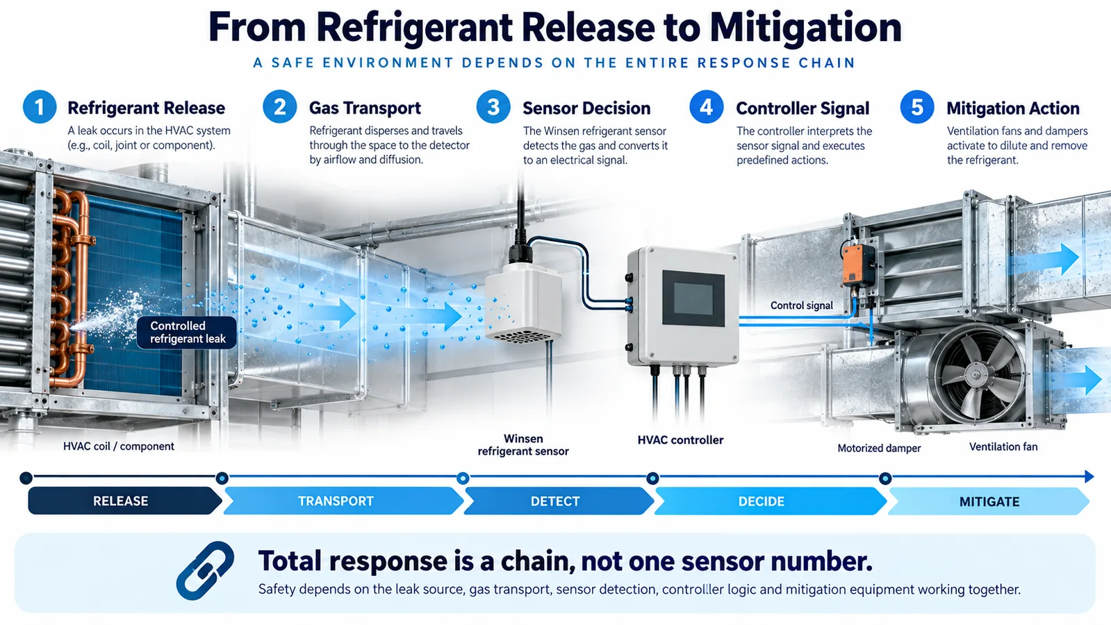
Refrigerant detection is often discussed as if response time were a single number printed in a sensor data sheet. It is not. In an HVAC safety function, the elapsed time that matters begins when refrigerant starts escaping and ends only when the intended mitigation has taken effect. Between those two events are gas transport, enclosure exchange, sensor physics, signal filtering, communications, controller logic, relay or network actuation, and the physical response of fans, dampers, valves, or other equipment.
That complete chain is the refrigerant sensor response time budget. Treating it as a system budget changes both design and testing. It prevents an engineer from selecting a fast sensing element and then losing most of the available time in a stagnant sampling location, a long moving-average filter, a slow polling interval, or an actuator that is never checked for proof of operation.
This guide presents an engineering workflow for allocating, measuring, and validating the response-time budget in R32 and other refrigerant-detection applications. It is not a substitute for the applicable equipment standard, listing, product instructions, or authority-having-jurisdiction requirements. The project team must obtain the required system behavior from those controlled documents and then demonstrate that the production design meets it.
1. Define the two endpoints before assigning numbers
Every useful timing requirement needs an unambiguous start event and end event. “Responds in 30 seconds” is incomplete unless the engineering record says what starts the clock, where concentration is measured, what threshold applies, and what physical condition stops the clock.
A defensible start definition might be one of the following:
- initiation of a repeatable test-gas release at a specified location and mass-flow rate;
- arrival of a specified concentration at a reference point next to the detector inlet;
- creation of a controlled leak in a representative refrigerant circuit;
- application of a calibrated gas step directly to the sensor fixture during component characterization.
These definitions answer different questions. Direct application to the sensor characterizes the device and its filter. A release inside an indoor unit characterizes gas movement, placement, enclosure effects, and the control chain. Do not report one result as though it proves the other.
The end point also needs precision. It may be:
- the detector output crosses the alarm criterion;
- the controller recognizes a valid alarm;
- the mitigation output changes state;
- a fan reaches a defined airflow;
- a damper reaches a defined position;
- a valve is proven closed;
- the controlled space or enclosure reaches the required safe condition.
For most equipment decisions, the final physical action is more meaningful than a software bit. A relay command does not prove that a disconnected fan started. If the risk assessment depends on airflow, measure or prove airflow.
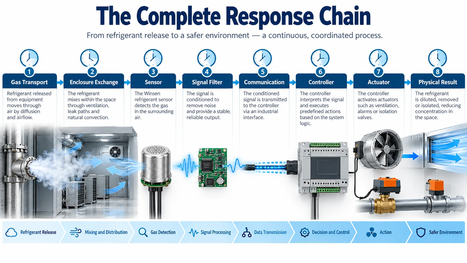
2. Model the complete response chain
The system delay can be organized as a sequence:
Ttotal = Ttransport + Tenclosure + Tsensor + Tfilter + Tcommunication + Tcontroller + Tactuator + Tphysical
The equation is a model, not a claim that every term is independent. Some stages overlap. For example, the sensor is already processing while concentration is still rising, and a fan may begin accelerating while a damper is moving. Nevertheless, separating the terms is valuable because it identifies ownership and test methods.
Create a budget table with at least these columns:
| Stage | Responsible owner | Design allocation | Worst-case basis | Verification method |
|---|---|---|---|---|
| Gas transport | mechanical / airflow | project-defined | worst release and operating state | representative release test |
| Detector enclosure exchange | detector integration | project-defined | blocked or weak flow path | inlet step / enclosure test |
| Sensor and filtering | sensor / firmware | project-defined | tolerance, temperature, aging | calibrated gas step |
| যোগাযোগ | controls | project-defined | maximum poll and retry interval | timestamped bus test |
| Controller logic | controls | project-defined | task scheduling and debounce | software/hardware-in-loop |
| Actuator command | equipment controls | project-defined | relay, network, drive latency | timestamped output test |
| Physical mitigation | mechanical | project-defined | cold start, low voltage, load | airflow/position feedback |
The actual allocations must come from the applicable requirement and the system safety analysis. An illustrative table is useful for design discussions, but it must never be copied into a product specification without evidence.
3. Gas transport usually contains the largest uncertainty
Gas cannot be detected before it reaches the inlet. The transport interval depends on release momentum, refrigerant state, local geometry, temperature, buoyancy, mixing, fan status, leakage through seams, and nearby obstructions. Refrigerant vapor density is relevant, but the rule “put the sensor low” is not a complete placement method. A high-velocity jet or an operating blower can carry a release across or upward through an enclosure. When the blower stops, the same gas can follow a different path and accumulate in a lower pocket.
Build a release-location map from real circuit features:
- service valves and access ports;
- field joints and flare connections;
- distributor and header joints;
- coil return bends;
- pressure switches and transducers;
- brazed transitions;
- compressor and accumulator connections;
- tubing locations vulnerable to vibration or abrasion.
Cross that map with operating states. At minimum, evaluate fan on, fan off, cooling, heating, defrost, standby, startup, shutdown, and service-panel removed if that condition changes the flow path. A detector location that is excellent during rated airflow can be slow when the unit is idle.
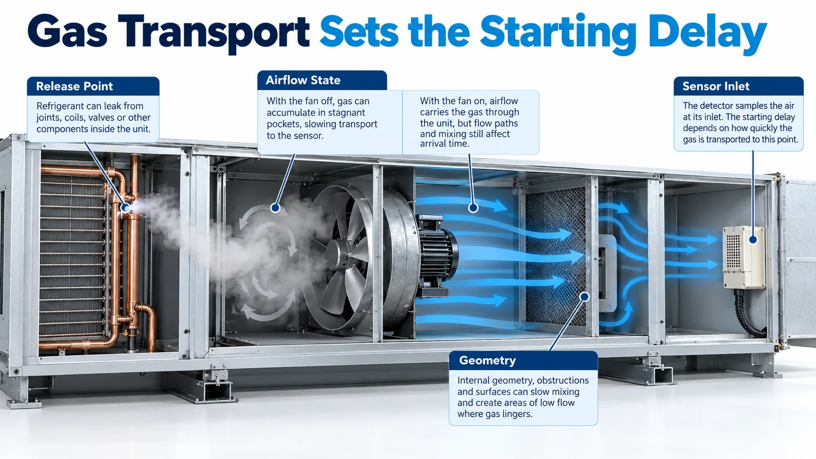
Transport validation should use more than one release point. Select the points that challenge the candidate detector location, not only the easiest or closest connection. If multiple circuit compartments are substantially isolated, one sensing point may not cover all of them. The budget exercise should reveal that architectural issue before late compliance testing.
4. Separate enclosure exchange from sensor response
An OEM may mount a sensing module behind a grille, in a plastic pocket, on a printed-circuit enclosure, or inside a secondary protective cover. Those features change the rate at which gas reaches the sensing element. A hydrophobic membrane, dust screen, tortuous path, or small inlet can improve environmental robustness while adding exchange delay.
Characterize the bare module and the final installed assembly separately. If the module meets its component target but the assembled product does not, the integration path—not necessarily the sensing element—is the problem.
Check for:
- foam seals that cover the intended inlet;
- wire bundles or labels placed across openings;
- an inlet facing a dead wall with insufficient clearance;
- dust filters with uncontrolled replacement grade;
- water shields that trap a stagnant gas volume;
- condensate or oil that can wet a membrane;
- insect screens or field-applied mesh;
- paint, insulation, or sealant introduced after qualification.
Make critical inlet geometry visible on drawings and manufacturing controls. A later cost-reduction change to a cover can silently consume the response-time margin.
5. Understand what the sensor time constant actually represents
Manufacturers may characterize response using a concentration step at controlled temperature and humidity. The reported metric may be T50, T63, T90, time to a threshold, or another definition. These are not interchangeable.
- T50 is the time to reach 50 percent of the final indicated change.
- T63 is associated with one time constant in a simple first-order model.
- T90 is the time to reach 90 percent of the final indicated change.
- Alarm response is the time to cross a configured criterion and depends on the applied concentration and logic.
For a threshold-based safety function, the time to alarm under the relevant concentration profile is usually more useful than a generic T90 value. Read the test conditions behind any data-sheet number. A high gas step applied directly to the inlet can cross an alarm threshold much sooner than a gradual field release.
Temperature, supply tolerance, contamination, aging, manufacturing variation, and calibration strategy can change the response. Use the worst supported operating conditions in the budget and maintain production controls that preserve them.
6. Digital filtering is a safety parameter
Signal filtering reduces noise and nuisance alarms, but it also adds delay. Common mechanisms include moving averages, exponential filters, consecutive-sample requirements, threshold persistence timers, hysteresis, and multi-stage confirmation logic.
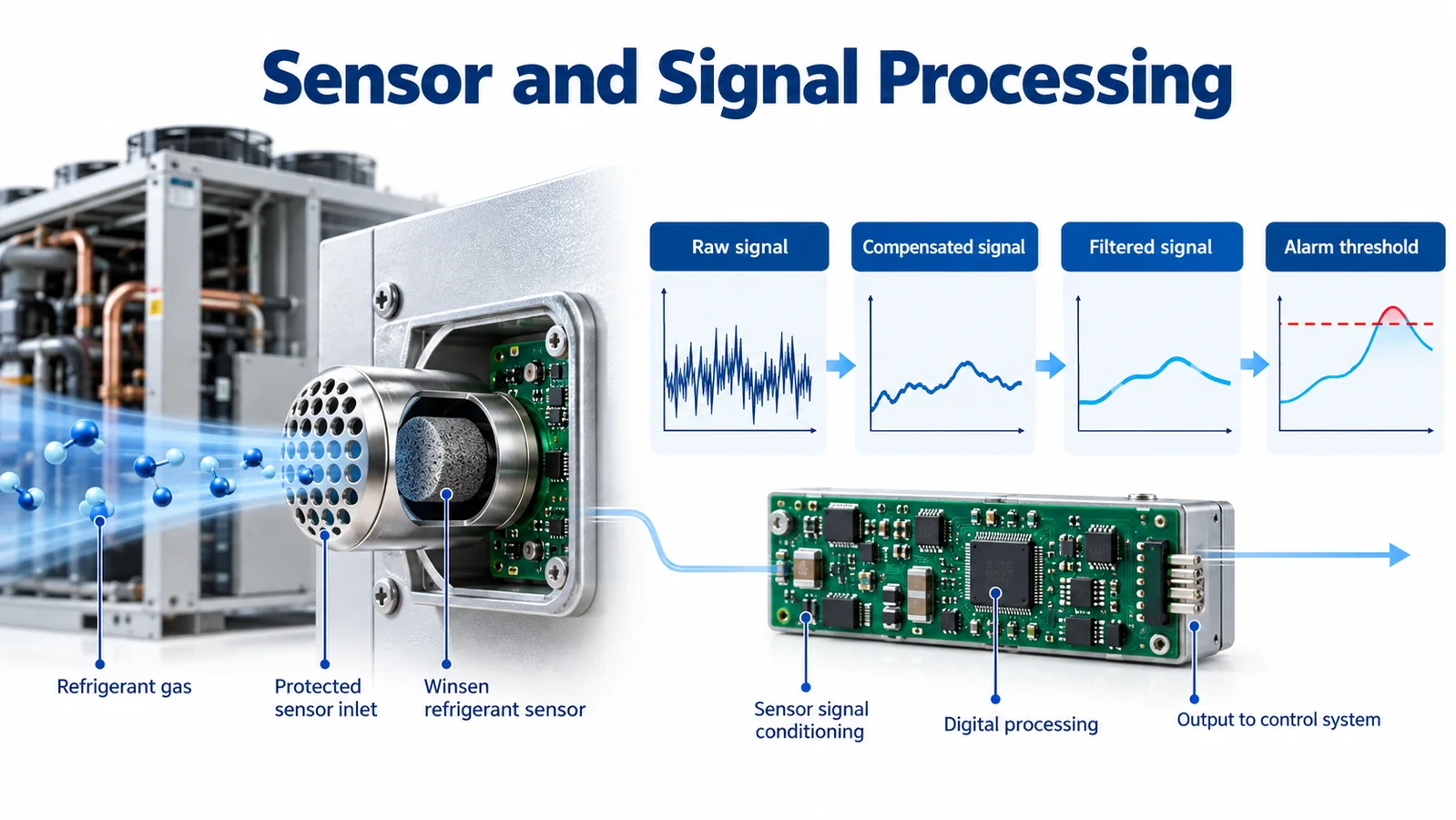
Document the signal path explicitly:
- raw optical or sensing measurement;
- compensation and validity checks;
- internal digital filter;
- concentration or state output;
- controller-side smoothing;
- alarm threshold and persistence;
- alarm latch or clear logic.
Two teams can unintentionally filter the same signal. The sensor supplier may average samples, and the equipment controller may apply another rolling average. The combined delay can be much longer than either owner expects. Capture firmware revision, filter coefficients, sampling interval, threshold, hysteresis, and persistence time in configuration control.
Do not solve a nuisance alarm by simply extending a delay until the symptom disappears. Investigate the exposure, placement, electrical noise, or interference mechanism. Any filter change must be re-entered into the budget and revalidated.
7. Budget communication latency with worst-case scheduling
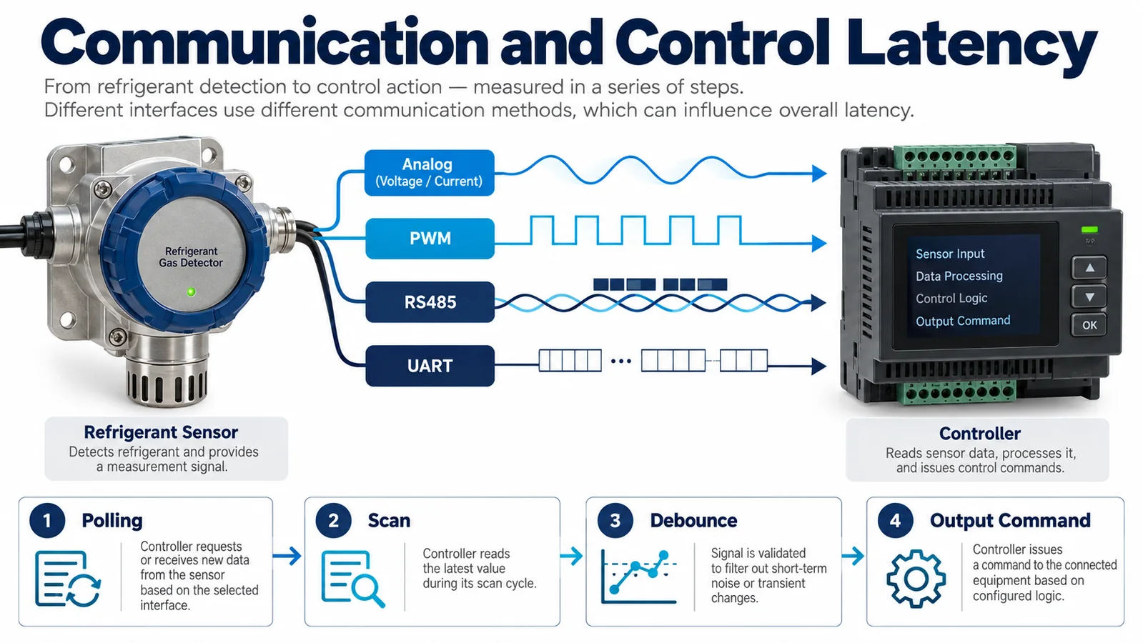
Analog, PWM, UART, RS485, and other interfaces have different timing behavior, but no interface is inherently fast unless the complete implementation is specified.
For a polled digital bus, include:
- sensor update interval;
- controller polling interval;
- worst phase alignment between update and poll;
- bus queue and task scheduling;
- timeout setting;
- permitted retries;
- error recovery;
- gateway or protocol conversion;
- stale-data recognition.
If a sensor updates just after the controller polls, the controller may wait nearly a full poll period. A retry strategy can add more delay. A gateway can buffer or resample data. Measure at the final controller, not only at a bench terminal.
For analog signals, include sensor output filtering, ADC sampling, input-module filtering, scan time, scaling, and threshold logic. For PWM, include frame period and the number of frames needed to declare a valid state. For a relay or discrete alarm output, include internal alarm processing and input debounce.
Use monotonic timestamps from synchronized acquisition channels whenever possible. Logging devices with unrelated clocks can create apparent negative or inconsistent delays.
8. Controller logic must distinguish alarm, fault, and invalid data
The controller should not treat every non-normal input as the same event. A detected refrigerant alarm, an internal detector fault, a communication timeout, a startup warm-up state, and invalid or stale data may require different annunciation and mitigation behavior.
Define:
- the exact input that declares alarm;
- whether the alarm is latched;
- the reset conditions and authority;
- the required response to detector fault;
- the maximum age of acceptable data;
- behavior during startup and firmware update;
- behavior after communication loss;
- priority if alarm and fault occur together;
- power-loss and brownout behavior.
Controller scan time is often small, but supervisory logic can add seconds through debounce, voting, timers, or state transitions. Review the actual executable path. A specification saying “on alarm, start fan” does not reveal whether a 10-second validation timer runs first.
9. Include actuator and physical mitigation time
The electrical command is not the end of the safety chain. Contactors close, drives initialize, motors accelerate, dampers travel, valves move, and airflow builds. At low temperature or low supply voltage, those actions may be slower. Mechanical loads and dirty filters can also change the result.
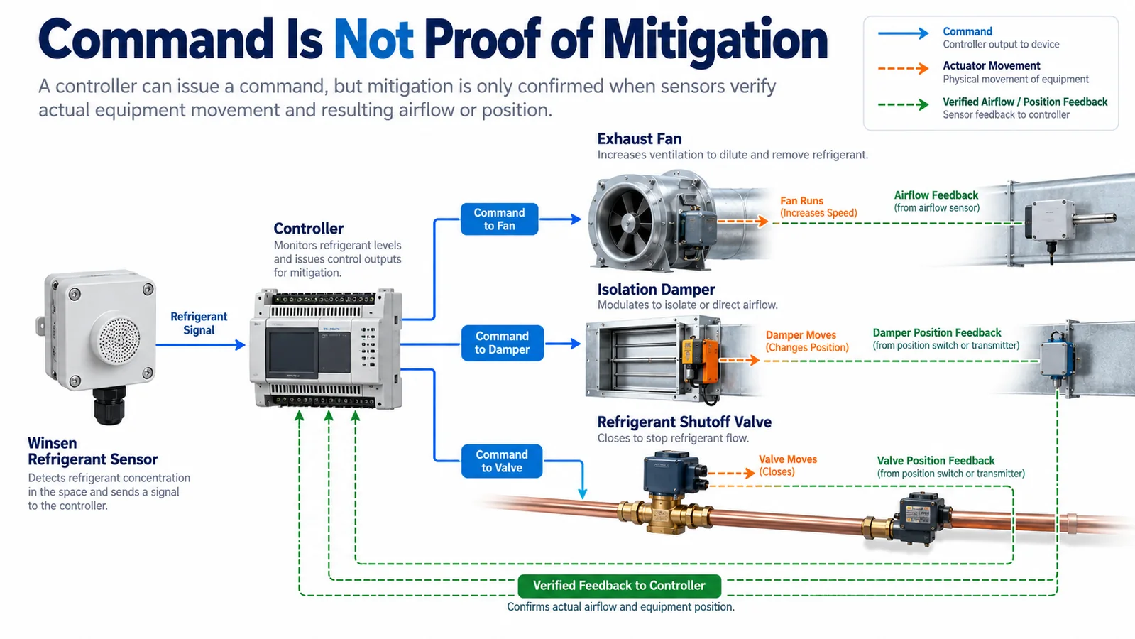
If the safety concept relies on dilution airflow, decide what proves it:
- fan command only;
- contactor auxiliary contact;
- motor current;
- drive run status;
- pressure differential;
- airflow switch;
- measured airflow.
Each option proves a different fact. A drive run bit does not necessarily prove the airflow assumed by the mitigation calculation. Select feedback consistent with the hazard analysis and applicable requirements.
Measure actuator time across the permitted operating range and after realistic standby. A motor starting from rest can differ from a continuously running fan. A damper with a 90-second stroke cannot support a 30-second physical end point unless the design requires only partial travel and proves it.
10. Allocate margin rather than spending the requirement exactly
A robust budget contains explicit margin for variation and uncertainty. Do not allocate every available second to nominal stage values. Consider:
- sensor production tolerance;
- temperature and humidity extremes;
- refrigerant concentration profile;
- aging and contamination;
- supply-voltage tolerance;
- bus traffic and task scheduling;
- actuator wear;
- filter loading;
- installation variation;
- measurement uncertainty.
The budget owner should know whether each figure is a maximum specification, a measured worst case, a statistical estimate, or a placeholder. Color coding can help during development, but the released record needs objective evidence and revision traceability.
Avoid adding worst cases blindly if stages overlap; that can make the model unrealistically conservative. Conversely, avoid combining nominal values and calling the result worst case. Where interaction is significant, run integrated tests at combined challenging conditions.
11. Build a synchronized validation method
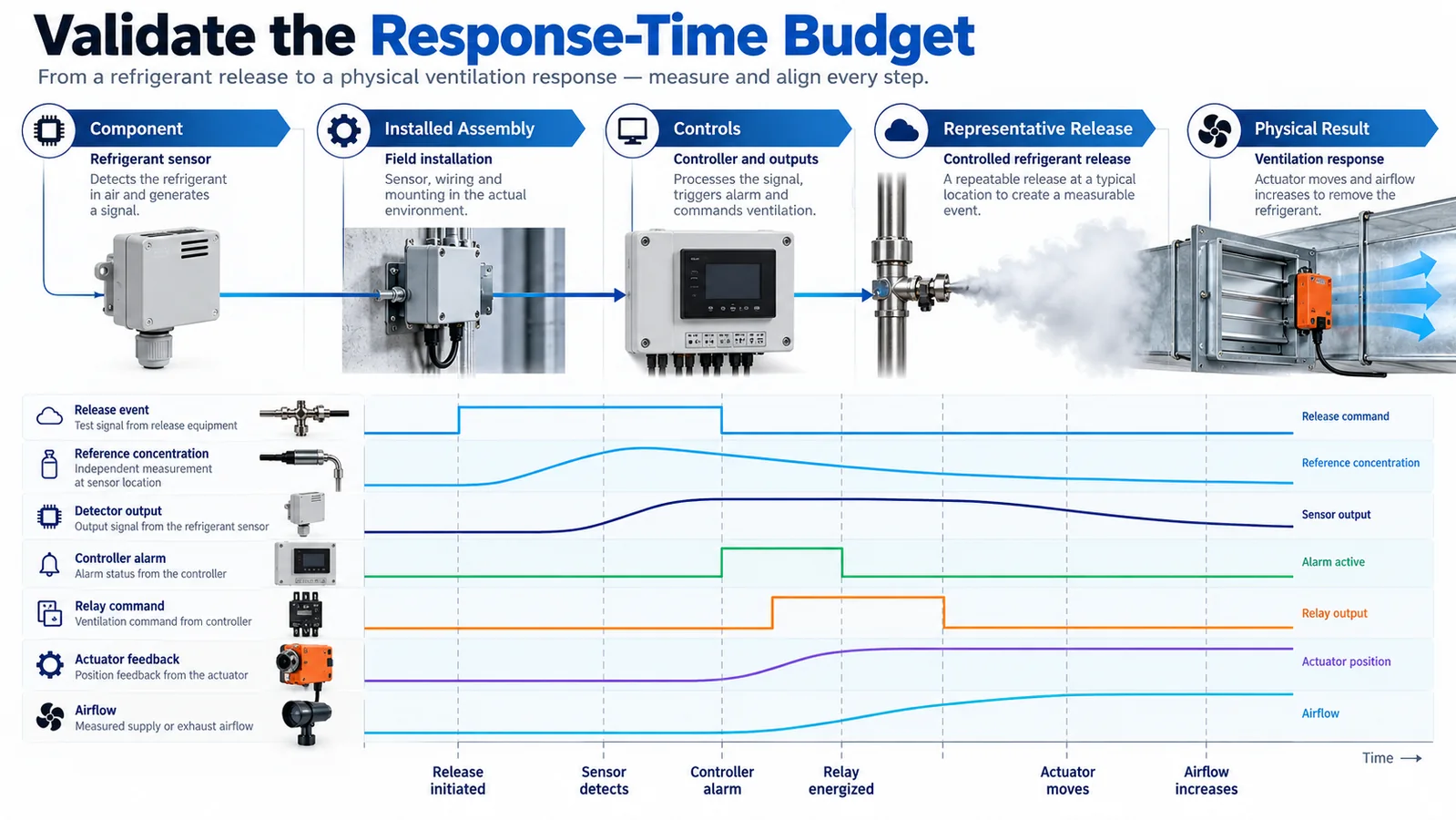
A strong test records the complete chain with enough time resolution to identify every transition. A typical acquisition set includes:
- release valve command or mass-flow trace;
- reference gas concentration near the detector inlet;
- detector raw or reported output;
- detector alarm state;
- bus message timestamps;
- controller alarm bit;
- physical output voltage or contact state;
- actuator feedback;
- airflow, damper position, or valve position.
Define sensor placement for the reference instrument carefully. A reference probe far from the product inlet measures a different concentration history. Its own response time and tubing delay must be characterized or corrected.
Run repeated trials. Random variation in release initiation, fan phase, network polling, and actuator start can hide the true worst case. Record all raw data, configuration versions, ambient conditions, release details, and test-fixture geometry.
Recommended test layers are:
- Component step test — characterize module, filter, threshold, and interface.
- Installed assembly test — include cover, inlet, and equipment mounting.
- Controls integration test — include production controller, bus, and outputs.
- Representative release test — challenge transport and operating states.
- Physical mitigation test — prove the final airflow, position, or isolation result.
12. Test failure cases, not only the happy path
A budget review should expose conditions in which the chain stops or becomes slower:
- detector disconnected;
- data frozen at the last valid value;
- corrupted frame or bad checksum;
- bus saturated or gateway offline;
- controller task delayed;
- output relay welded or open;
- fan cannot start;
- damper stalls;
- feedback switch misadjusted;
- detector inlet obstructed;
- low-voltage supply during startup;
- simultaneous alarm and detector fault.
Determine which failures are detected, how quickly they are detected, what signal is sent, and what fallback action is required. The fault-detection interval belongs in its own safety analysis; it should not be confused with the refrigerant-alarm response time.
13. Use change control to preserve response performance
Response performance is a system property, so many ordinary changes can affect it:
- new sensor firmware;
- revised filter coefficient;
- alternate detector supplier;
- changed inlet grille;
- new gasket or foam;
- moved wire harness;
- new controller scan schedule;
- added network traffic;
- different drive or damper actuator;
- altered fan ramp profile;
- changed refrigerant charge or circuit layout.
Maintain a response-time impact checklist in engineering change control. Low-risk changes may need a targeted regression test; architectural changes may require full integrated validation. Keep the original time histories so a new design can be compared with the qualified baseline.
14. Review the budget with a worked engineering record
For each limiting scenario, create a one-page timing record. Start with the equipment variant, refrigerant circuit, release point, fan and damper states, ambient condition, detector revision, controller software and actuator configuration. Then list the measured timestamps and the uncertainty of each channel. The record should show both the design allocation and the observed value so reviewers can see where margin exists.
Do not mix data from unrelated tests to create an unrealistically attractive total. A transport time measured with the fan at nominal speed should not be combined with an actuator time measured at a low-voltage corner and presented as one verified scenario. Either test the complete chain together or clearly state which bounded component results support the combined worst-case argument.
When a stage exceeds its allocation, avoid moving the excess silently into another line. Decide whether the total requirement and margin still hold, whether the allocation was unrealistic, or whether the design needs change. The budget is a coordination tool, so every revision should identify its technical reason and affected test evidence.
15. Control measurement uncertainty and data alignment
Timing accuracy is often better than concentration accuracy, but both matter. Characterize data-acquisition sample interval, channel skew, reference-sensor response, tubing delay, release-valve delay and actuator feedback tolerance. If video is used to observe a damper, synchronize it with the electronic traces using a visible or logged event.
Use raw, monotonic timestamps rather than screenshots as the master record. A trend display can interpolate points or resample slow values, hiding the actual threshold crossing. Preserve original files, calibration certificates, scripts or spreadsheet formulas used for analysis, and the revision of the threshold algorithm.
Report how crossing time is selected when signals are noisy. Consistent rules—such as first sustained crossing under the released persistence logic—make comparisons reproducible. Do not hand-pick the fastest sample from repeated oscillations.
16. Use timing margin as a production health indicator
Once the design is qualified, selected end-of-line or audit tests can monitor whether timing is drifting. These checks need not reproduce every certification scenario, but they should be sensitive to blocked inlets, wrong firmware, excessive filtering, communication misconfiguration and slow actuators.
Trend the measured stages separately. A stable total can hide opposite changes, such as faster transport but slower filtering. Supplier changes, production tooling, software updates and field complaint data should feed the same timing review. If margin approaches the project action limit, investigate before a formal requirement is exceeded.
17. Product integration example: ZRT510 R32
For R32-specific equipment development, the Winsen ZRT510 R32 module is one product family that may be evaluated. The current product information describes NDIR sensing and lists PWM, RS485, and UART interface options. The integration team must confirm the exact ordered variant, electrical limits, update behavior, warm-up, diagnostic states, alarm strategy, and response characteristics in the controlled data sheet before design release.

Do not infer system compliance from the module alone. Gas transport, final enclosure, controller logic, actuator performance, equipment construction, and the applicable certification path remain responsibilities of the complete equipment design.
Engineering checklist
Before freezing the response-time design, confirm that the team can answer every item below:
- What exact event starts the clock?
- What physical condition ends the clock?
- Which requirement controls the total time?
- Which stages are included in the budget?
- Is transport evaluated for every credible release zone and operating state?
- Is the final detector cover included in testing?
- Are sensor filtering and controller filtering both documented?
- Is worst-case communication scheduling included?
- Are alarm, fault, warm-up, and stale-data states distinguished?
- Is the physical mitigation action measured or proven?
- Is adequate margin retained?
- Are timestamps synchronized and reference-instrument delays known?
- Have failure cases been tested?
- Does change control identify every parameter that can consume timing margin?
উপসংহার
A fast refrigerant sensor is valuable, but it does not guarantee a fast safety response. The useful engineering quantity is the time from a defined release event to a verified physical mitigation result. By breaking that interval into transport, enclosure exchange, sensing, filtering, communications, controller, actuator, and physical-action stages, teams can assign ownership and find hidden delays early.
The resulting budget should be linked to controlled requirements, supported by synchronized measurements, challenged across operating states, and protected by change control. That discipline produces a refrigerant-detection system whose timing can be explained and reproduced—not merely a sensor with an attractive data-sheet number.
For sensor selection or integration review, provide the target refrigerant, expected concentration range, interface, equipment geometry, operating states, intended mitigation action, and required timing endpoint. Winsen can then help identify candidate modules and the evidence still needed at equipment level.
